Google Sheet Pivot Table Calculated Field

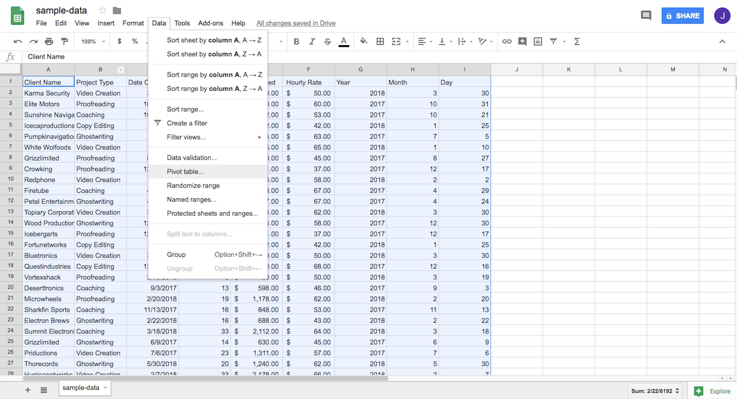
Google Sheet Pivot Table Calculated Field - Highlight the data range and from the file menu select “insert” > “pivot table”. In this example we will highlight cells a1 to c7. Select ‘calculated field’ from the dropdown menu. Select the data range to be implemented in the pivot table. Web how to add a calculated field in pivot table in google sheets 1. In the pivot table editor, click on the ‘add’ button next to ‘values’. How to add calculated field in pivot table step 1: In the file menu, select insert. Preparing a pivot table in this sample data, i can group the first two columns and they are date (column a) and. We start the same way by adding a calculated field from the values section and naming it ‘max units sold’.

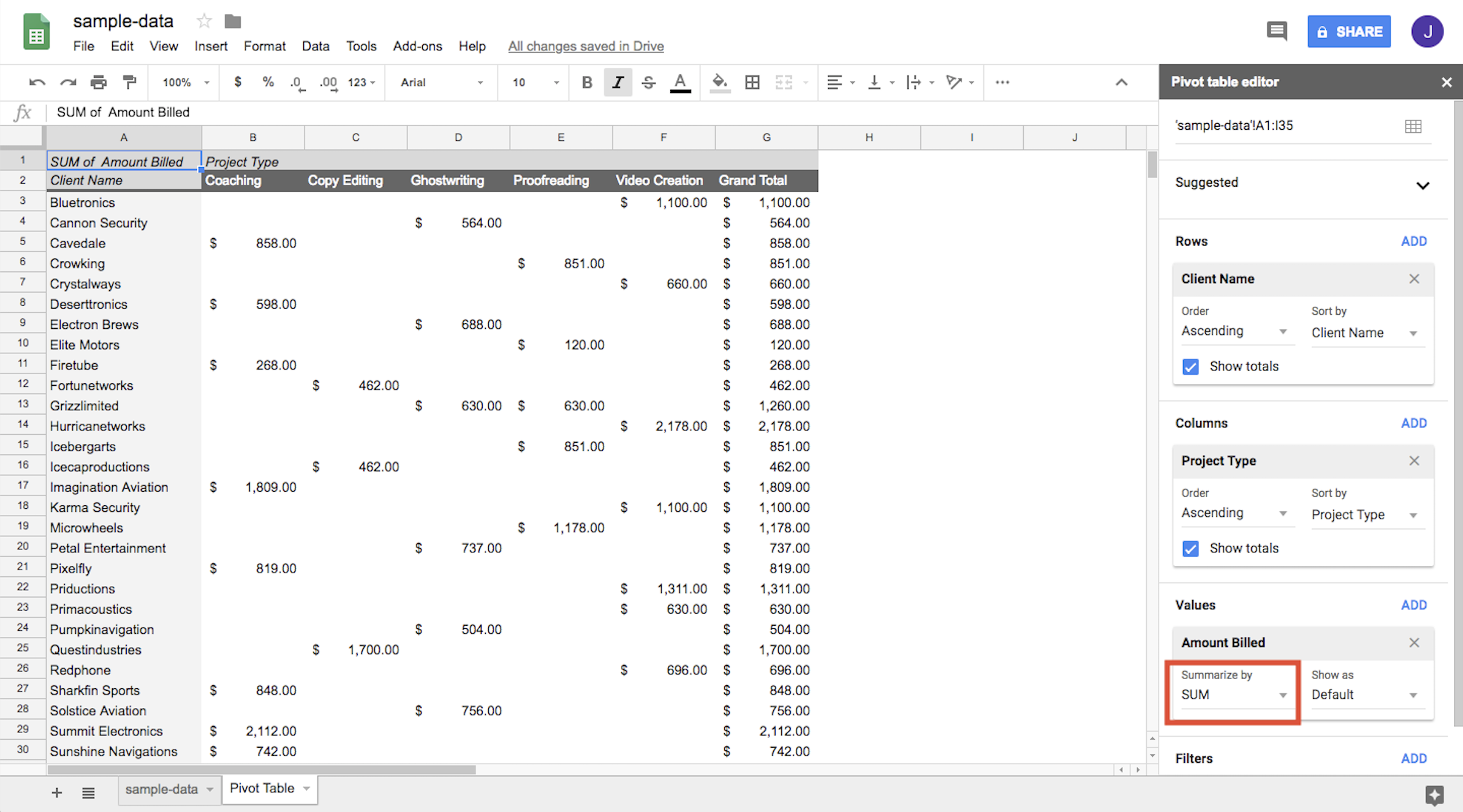
Highlight the data range and from the file menu select “insert” > “pivot table”. Web how to add a calculated field in pivot table in google sheets 1. Preparing a pivot table in this sample data, i can group the first two columns and they are date (column a) and. How to add calculated field in pivot table step 1: =max ('sold unit') usually, this is the step where we get the. Enter the data first, let’s enter the following data that shows the total revenue generated by certain products. We start the same way by adding a calculated field from the values section and naming it ‘max units sold’. In the pivot table editor, click on the ‘add’ button next to ‘values’. In this example we will highlight cells a1 to c7. Select the data range to be implemented in the pivot table.

How to add calculated field in pivot table step 1: Preparing a pivot table in this sample data, i can group the first two columns and they are date (column a) and. Select ‘calculated field’ from the dropdown menu. Web how to add a calculated field in pivot table in google sheets 1. In the pivot table editor, click on the ‘add’ button next to ‘values’. Select the data range to be implemented in the pivot table. Web you can add a calculated field to your pivot table by following the steps below: In the file menu, select insert. Highlight the data range and from the file menu select “insert” > “pivot table”. Enter the data first, let’s enter the following data that shows the total revenue generated by certain products.

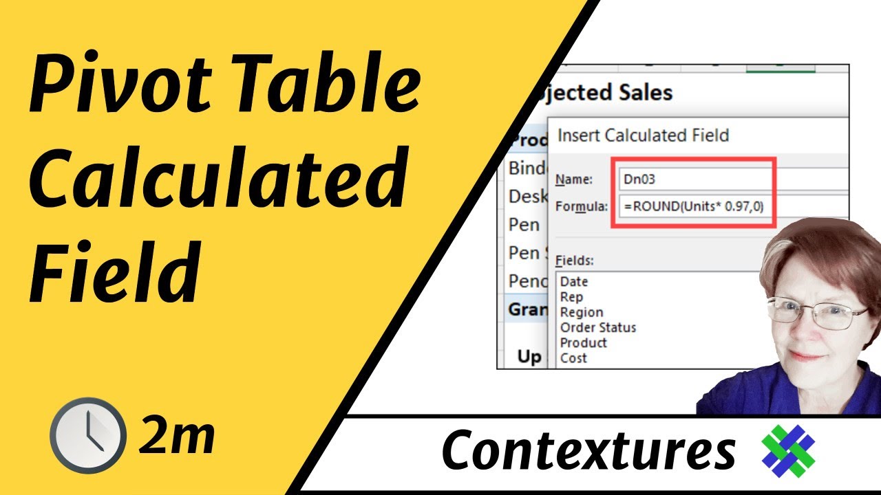
Create a Calculated Field in Excel Pivot Table YouTube

In the file menu, select insert. Preparing a pivot table in this sample data, i can group the first two columns and they are date (column a) and. Select the data range to be implemented in the pivot table. We start the same way by adding a calculated field from the values section and naming it ‘max units sold’. Highlight.

Use calculated fields in a Google Sheets pivot table to count rows

Select ‘calculated field’ from the dropdown menu. =max ('sold unit') usually, this is the step where we get the. Enter the data first, let’s enter the following data that shows the total revenue generated by certain products. Web you can add a calculated field to your pivot table by following the steps below: Preparing a pivot table in this sample.

How to Format Pivot Tables in Google Sheets

Select ‘calculated field’ from the dropdown menu. Web how to add a calculated field in pivot table in google sheets 1. In this example we will highlight cells a1 to c7. =max ('sold unit') usually, this is the step where we get the. In the pivot table editor, click on the ‘add’ button next to ‘values’.

arrays Pivot table Display growth rate with calculated field in

In this example we will highlight cells a1 to c7. Select the data range to be implemented in the pivot table. In the file menu, select insert. Preparing a pivot table in this sample data, i can group the first two columns and they are date (column a) and. =max ('sold unit') usually, this is the step where we get.

Googlesheets How to reuse calculated field Valuable Tech Notes

Select the data range to be implemented in the pivot table. Select ‘calculated field’ from the dropdown menu. In the file menu, select insert. Highlight the data range and from the file menu select “insert” > “pivot table”. In this example we will highlight cells a1 to c7.

Google Sheets Create Pivot Tables and Charts YouTube

Select ‘calculated field’ from the dropdown menu. Enter the data first, let’s enter the following data that shows the total revenue generated by certain products. How to add calculated field in pivot table step 1: =max ('sold unit') usually, this is the step where we get the. Preparing a pivot table in this sample data, i can group the first.

Excel Pivot Tables Cheat Sheet lasopapac

Highlight the data range and from the file menu select “insert” > “pivot table”. We start the same way by adding a calculated field from the values section and naming it ‘max units sold’. Select ‘calculated field’ from the dropdown menu. In this example we will highlight cells a1 to c7. =max ('sold unit') usually, this is the step where.

How To Add Pivot Table Calculated Field in Google Sheets Sheets for

Web how to add a calculated field in pivot table in google sheets 1. Select the data range to be implemented in the pivot table. How to add calculated field in pivot table step 1: Select ‘calculated field’ from the dropdown menu. Highlight the data range and from the file menu select “insert” > “pivot table”.

How To Create A Simple Pivot Table In Excel Knowl365 Riset

Web how to add a calculated field in pivot table in google sheets 1. Select ‘calculated field’ from the dropdown menu. In the file menu, select insert. Preparing a pivot table in this sample data, i can group the first two columns and they are date (column a) and. Select the data range to be implemented in the pivot table.

Vincent's Reviews How to Use Pivot Tables in Google Sheets

Enter the data first, let’s enter the following data that shows the total revenue generated by certain products. We start the same way by adding a calculated field from the values section and naming it ‘max units sold’. Highlight the data range and from the file menu select “insert” > “pivot table”. Select the data range to be implemented in.

Web You Can Add A Calculated Field To Your Pivot Table By Following The Steps Below:

Enter the data first, let’s enter the following data that shows the total revenue generated by certain products. =max ('sold unit') usually, this is the step where we get the. In this example we will highlight cells a1 to c7. In the pivot table editor, click on the ‘add’ button next to ‘values’.

Preparing A Pivot Table In This Sample Data, I Can Group The First Two Columns And They Are Date (Column A) And.

Select ‘calculated field’ from the dropdown menu. In the file menu, select insert. Select the data range to be implemented in the pivot table. We start the same way by adding a calculated field from the values section and naming it ‘max units sold’.